Distance Tables Part 2: Lee's Visibility Graph Algorithm
In part 1 I defined that the problem is to implement a visibility graph algorithm with a time complexity better than . I chose to implement D.T. Lee’s visibility graph algorithm which runs in time. My Python implementation is available on Github as a open source package, Pyvisgraph.
The key sources I found and used in my research to implement Lee’s algorithm were as follows:
- Kitzinger, J. (2003). The visibility graph among polygonal obstacles: A comparison of algorithms
- Coleman, D. (2012). Lee’s O(n^2 log n) Visibility Graph Algorithm Implementation and Analysis
- Berg, M. D. (2008). Computational geometry: Algorithms and applications. Berlin: Springer.
- http://cs.smith.edu/~streinu/Teaching/Courses/274/Spring98/Projects/Philip/fp/algVisibility.htm
Lee’s algorithm was the first non-trivial solution to the visibility problem. He wrote this algorithm as part of his 1978 Ph.D. dissertation. Faster solutions were created after that, the fastest being the Ghosh and Mount approach running in time. There are two key reasons I chose not to implement these faster algorithms:
-
Human complexity: The Gosh/Mount algorithm is much more difficult to implement than Lee’s. For my use case, it is not critical to get the extra reduction in time complexity as I will build the visibility graph once, save it and load for subsequent use.
-
Reuse: I want to be able to not just find the shortest path between Port A and Port B, but also from any position to any position. This so I can update the route of a vessel that is in the middle of the ocean to its destination. Once the visibility graph is built, I need to be able to update it with a new point. This is easy to do with Lee’s algorithm in time, but not possible with the Gosh/Mount algorithm.
Lee’s visibility graph algorithm
We are still going to need the first two for loops as in the naïve solution
detailed in part 1; Lee’s approach saves us running time by reducing the number of
edges we need to check for each pair of points. That part of Lee’s algorithm runs
in time, leaving a total running time of .
visibility_graph(S <-- disjoint polygonal obstacles)
    G <-- all vertices of S
    VG -> empty visibility graph
    for each vertex v in G                                        #O(n)
        do VG <-- visible_vertices(v,S)                           #O(n log n)
    return VG
Before we look at the visible_vertices function, a key concept to understand
in Lee’s algorithm is the scan line.
Let’s say we are checking which points are visible from point s. To do this
we need to visit each of the points a through f. The way we are going to visit
the points is in a counter clockwise circle. We are going to use Lee’s scan line
for this, which is a half-line. Conceptually the scan line has its origin at
point s, pointing to the right (parallel to the x-axis) and moves counter clock
wise until it hits a point to check for visibility.
Together with the scan line we are going to keep a ordered list of edges that
we will need to use when we visit each point. we call this the open_edges
list. This list will be used to check for point visibility.
Once the scan line hits a point, the algorithm is going to work some magic on
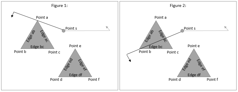
the edges incident on the point. Take figure 1: the first point the scan line
will hit is point a, which has two edges (edge ab and edge ac). what
we do is check if each edge is on the “counter clock wise” side of
the scan line. I.e., when the scan line continues moving, will it intersect any
of those edges? In the case of point a, both edges are on the CCW side and will
be added the open_edges list I mentioned we are tracking.
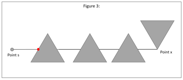
Lets continue the scan line to point b (figure 2). Now, edge ab is
on the clock wise side of the scan line and it will never be intersected by the
scan line again. This means we are free to completely ignore that edge for all
unvisited points and we can remove it from the tracking open_edges list.
edge ac is still partially on the CCW side and as the scan line continues to
move, it will continue to intersect edge ac, so it stays in the list.
edge bc should now be added to open_edges as it is on the CCW side and will
be intersected by the scan line. So for each point the scan line visits, we
check the edges incident at that point. If the edge is on the CCW side, we add
it to open_edges. If the edge is on the CW side, we remove it from open_edges.
Lets now discuss visibility, using figure 1 and 2. When the scan line visits
point a, it will check the open_edges list to see if there are any edges
that could possibly block visibility. At point a there are none so a is
visible. Moving to point b, open_edges contains edge ac and the line from
point s to point b intersects edge ac. point b is therefore not visible.
As illustrated, what the scan line allows us to do is ignore edges that are no
longer an issue, i.e. edges that can no longer block visibility of the next points
to visit. When the scan line moves on to point c, d, e and f, it will never
have to consider the edges that it has already passed, like edge ab. The naïve
algorithm would have to check all edges, Lee’s algorithm only checks relevant
edges.
As a matter of fact, we only need to check the closest open_edges edge.
Take figure 3 below: when the scan line visits point x, open_edges will
contain all the left and right edges of the three triangles. We don’t need to
loop through open_edges and check if we intersect an edge, we only need to
check the edge with the closest intersect point from s (i.e. the left most edge
in this case).
To achieve this, we need to keep open_edges ordered by the intersect distance
on the scan line from s. We achieve this using a binary search tree, which
allows us to look up the closest open edge in time. Implementing
this is not straight forward and will be the topic of Part 3.
visible_vertices(v, S):
    1. sort the vertices of the obstacle polygons according to the
    counter clock wise angle the half line from v to each vertex makes
    with the x-axis. In the case of ties, vertices closer to v should
    come first. Let w_i, ..., w_n be this list.
    2. let s be the scan line (half line) starting at v, parallel with
    the x-axis, extending to positive infinity. Check all edges of
    S for intersection with s and store intersected edges in a binary
    search tree T.
    3. W <-- empty list of visible vertices
    4. for i <-- 1 to n vertices
    5.     do if visible(w_i) then add w_i to W
    6.     Insert into T the edges incident to w_i that lie on the counter
           clock wise side of scan line s.
    7.     Delete from T the edges incident to w_i that lie on the clock
           wise side of scan line s.
    8. Return W
In step 1, we order all the points we are going to visit in the order the scan line will hit the points, moving in a counter clock wise direction.
In step 2, we initialize open_edges. It is important to do this before we start
visiting all the points; figure 3 illustrates the reason for this. In figure 3,
the first point the scan line hits is x. If we do not perform step 2.,
open_edges will be empty and we would think that x is visible. So in the
initialization step, we need to check all obstacle edges and store the edges
that intersect the horizontal scan line. This step takes
(checking n edges, where inserting into the binary search tree costs
).
In steps 4 to 7, we visit each of the obstacle points and check for visibility.
We also perform the edge magic explained above, keeping our open_edges updated.
visible(w_i):
    1. If T is empty then return True
    2. else if the edge from v to w_i does not intersect the smallest
       (left-most) edge in T then return True
    3. else return False
In step 1, if there are no edges in open_edges, then w_i is visible. In
step 2, open_edges is not empty, so we need to check the “smallest” or edge
that has the shortest distance to the intersection point with v to w_i. In
a binary search tree, that will be the left-most node. If v to w_i
intersects this line, then w_i is not visible.
How to store and use the open_edges tree will be the subject of Part 3.