Distance tables tell you the distance from Port A to Port B in nautical miles. They are used extensively by practitioners in the shipping industry; in my company, we use distance tables to estimate the value of a potential voyage. When you are paid in dollars per ton of cargo transported, distance will decide if a voyage is profitable or not. Distance is also key to scheduling vessels, i.e. knowing when a vessel will or can arrive at a port.

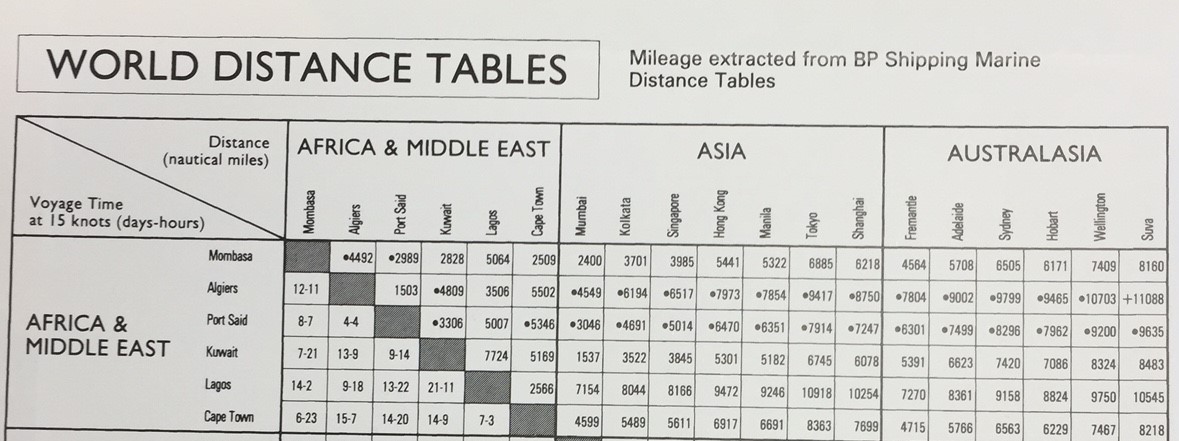
The above image is from my copy of Lloyd’s Maritime Atlas. We no longer look up distances in a book, but use commercial software that allows us to input origin, destination and any routing points. The output is the total distance and the route proposed. The reason I started researching distance tables is that I had written a Python script that scraped the GPS coordinates of our vessels and displayed them on a Matplotlib Basemap. I also added a visual of the route each vessel would take, by getting the coordinates manually from the commercial platform we use. This is tedious for 15 ships, so I wanted to find a solution to automate finding the voyage paths.

I started by asking a colleague (who is a Captain) how he thought the distance tables were made. He was sure each distance was manually calculated and that there was no algorithm behind it. Turns out he was in many cases right. The first distance tables were published by the BP Tanker Company in 1958¹ and all the distances were manually calculated. The second edition of the tables was printed in 1976. In 2000, ten ex. BP Masters decided to update the distance tables and make them available digitally. The update included taking into account the IMO Traffic Separation Scheme. It took them 4 years to complete this work (again, all manual calculations) and the tables were released in 2004 as AtoBviaC.

My use case does not need to be as accurate as the BP tables or other commercial software. I need to find the shortest path from port A to B, get the route coordinates and display it on a Basemap. The route doesn’t need to follow navigational rules as it will never be used for navigational purposes. It is purely for simple illustration of where our ships are heading.

My research therefore started from this perspective: find the shortest path in the presence of obstacles (the obstacles in this case will be shorelines). I already know shortest path algorithms (A* or Dijkstra’s), so I needed to figure out how to build the graph. Path finding is actually a common problem in robotics and my research led me to Chapter 15 of Computational Geometry: Algorithms and Applications. The graph I needed to build is called a Visibility Graph.

Visibility graphs & the naïve algorithm

Computational Geometry defines visibility graphs in the following way: Given a set $S$ of disjoint polygonal obstacles, we denote the visibility graph $G_{vis}(S)$. It’s nodes are the vertices of $S$ and there is an arc between vertices $v$ and $w$ if they can see each other, that is, if the segment $\overline{vw}$ does not intersect the interior of any obstacle in $S$.

To better understand the visibility graph, lets look at the naïve algorithm:

G <-- all vertices of S
VG <-- empty visibility graph
for each vertex v in G                                            #O(n)
    for each vertex w in {G - v}                                  #O(n)
        for each edge e in S                                      #O(e)
            if the arc from v to w does not intersect any edge e then
            vertex v and w are visible to each other
                VG <-- edge v to w

To build the visibility graph naïvely, we add all the vertices from our set of obstacles to visibility graph $G$. For each vertex $v$ in $G$, we check it against all the other vertices in $G$ to see which vertices are visible to $v$. To check if a vertex $w$ is visible, we need to check if the arc/edge from $v$ to $w$ intersects with any of the edges of the obstacles. If it doesn’t intersect any edges, $v$ is visible to $w$ and vice versa. There is no obstacle blocking the view between $v$ and $w$ and it can be used as part of a path.

The below video is a good example of a visibility graph being built:

A video showing the shortest path algorithm used on a visibility graph:

The Problem

The issue with the naïve algorithm is that it’s time complexity is $O(n^3)$. To put that in perspective, the shoreline obstacles I use contain 4999 vertices. That means this algorithms would, very roughly, run 125 billion commands (which takes several hours on my laptop).

The key problem to solve is therefore how to implement an algorithm that finds the visibility graph in better than $O(n^3)$ time. The algorithm I ended up researching and implementing was developed by D.T. Lee in his 1978 Ph.D. dissertation and was the first non-trivial solution to the visibility graph problem. His algorithm and runs in $O(n^2 log_2 n)$ time - that is 307 million commands instead of 125 billion - a huge improvement.

Lee’s visibility graph algorithm will be the subject of part 2 of this article series. My Python implementation is available on Github as a open source package, Pyvisgraph.